How do you win at slot machines? From one point of view, it is random whether you win or lose on each pull of the machine’s arm. On the other hand, if you understand how these machines work exactly, you could design a strategy to maximize your chance of winning. Unfortunately, designing such a strategy is difficult because it involves making very complicated decisions about when to pull the handle.
In this tutorial, I would like to show you how the methodology can help us answer some of these questions. For the purpose of illustration, we have picked a casino example:
Assume a Mathematician goes to Casino floor. He doesn’t have any prior information about the Math implemented by games developers in slot machines.

He will have no choice but to assume that winning probability of each slot machine is equal i.e. 50%, then he will assume that winning probability θ of each slot machine follows Beta distribution with hyperparameters α=β=2 as a Prior Belief.
Now if he gets some observed data D, he can estimate probabilistic model’s parameter θ (Winning Probability of Slot Machine) by using MLE (Maximum Likelihood Estimation) OR MAP (Maximum as Posteriori) as follows:

In order to compute MLE or MAP, he asks for Some data and somebody on the casino floor shares a small set of data with him as follows:
Slot Machine 1: Won 2 times when played only 3 Games.
Slot Machine 2: Won 101 times when played game for 168 times.
By intuition, not only him but anybody would also think “Slot Machine 2” is the special one, because getting 2 wins out of 3 plays on “Slot machine 1” could just happen by chance. But “Slot Machine 2” data doesn’t look like happening by chance.
Now, how to prove mathematically if the intuition is Correct?
He has an access to frequentist (MLE) approach and Bayesian Point Estimator approach (MAP).
Being a Mathematician, he knows that MLE will not work because of very small size of the observed Data.
So, he tries to use MAP because he has got some Data and also prior belief that winning probability of each slot machine follows Beta distribution with hyperparameters α=β=2.
Assuming that the results (k wins out of n plays) follow binomial distribution with the slot machine’s winning probability θ as its parameter.
The formula and results are as given below:

Slot Machine 1: (2+2–1)/(3+2+2–2) = 3/5 = 60%
Slot Machine 2: (101+2-1)/(168+2+2-2) = 102/170 = 60%
BAM! Unlike the intuition, estimated winning probability θ by MAP for these two slot machines are exactly same. Hence, Bayesian MAP estimators also didn’t help him determine which one is the special slot machine, which is likely to leave him wondering if the common human intuition about this is fake.
But really? Isn’t it looking obvious that “Slot Machine 2” is more likely to be the special one?
The mystery remained unsolved until he decided to move beyond MLE & MAP and decided to calculate full distribution, which is nothing but the Bayesian inference, which returns probability density (or mass) function.

To see if there really be no difference between Slot Machine 1 and Slot Machine 2, he calculates the posterior probability distribution, not only MAP estimates.
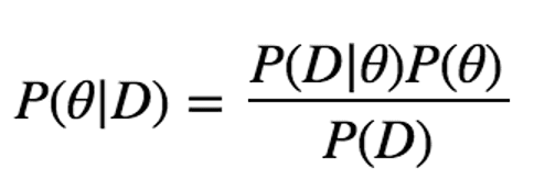
The posterior probability distribution P(θ|D) is calculated as below:

In Bayesian inference, we also need to calculate P(D) called marginal likelihood or evidence apart from calculating Likelihood and Prior in MAP. It’s the denominator of Bayes’ theorem and it assures that the integrated value of P(θ|D) over all possible θ becomes 1 (Sum of P(θ|D), if θ is a discrete variable).
P(D) is obtained by marginalisation of joint probability. When θ is a continuous variable, the formula is as below:

Considering the product rule

Now, put this into the original formula of the posterior probability distribution. Calculating below is the goal of Bayesian Inference.

How to calculate full distribution P(θ|D) in three parts?
#1: Likelihood, P(D|θ): It is the probability that data D is observed when parameter θ is given. For the slot machine 1, D is “2 wins out of 3 plays”, and parameter θ is the winning probability of Slot machine 1. As we assume that the number of wins follows binomial distribution, the formula is as below, where n is the number of plays and k is the number of wins.

#2: The prior probability distribution of θ, P(θ): It is the probability distribution expressing our prior knowledge about θ. Here, specific probability distributions are used corresponding to the probability distribution of Likelihood P(D|θ). It’s called conjugate prior distribution.
Since the conjugate prior of binomial distribution is Beta distribution, we use Beta distribution to express P(θ) here, incidentally it is also matching with prior belief of mathematician when he got on to the casino floor.
Beta distribution is described as below, where α and β are hyperparameters.

Now we got P(D|θ)P(θ) — the numerator of the formula — as below:

#3: Evidence, P(D): It is calculated as follows. Note that the possible range of θ is 0 ≤ θ ≤ 1.

With Euler integral of the first kind, the above formula can be deformed to:

Finally, we can obtain P(θ|D) as given below:

Expected A Posteriori (EAP):
The estimate by MAP is the mode of the posterior distribution but it didn’t solve his problem, therefore he is looking for other statistics for the point estimation, such as expected value of θ|D. The estimation using the expected value of θ|D is called Expected A Posteriori.

Let’s estimate the winning probability of the two slot machines using EAP. From the discussion above, P(θ|D) in this case is below:

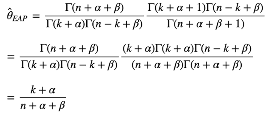
Thus, the estimate is described as below:

With Euler integral of the first kind and the definition of Gamma function, above formula can be deformed to below:

Hence, EAP estimate of Two slot machines winning probabilities with hyperparameters α=β=2 are below:
Slot Machine 1: (2+2)/(3+2+2) = 4/7 = 57.1%
Slot Machine 2: (101+2)/(168+2+2) = 103/172 = 59.9%
Hurray! The intuition is proved correct as “Slot Machine 2” has slightly higher winning probability than the “Slot machine 1”
In a similar way, you can solve real world problems without getting into the source code of the applications or even without knowing about the business rules/hand crafted logics implemented in the software.
This blog is authored by

Sukhdev Singh
Senior Director – Engineering, PureSoftware


